Reactive Programming helps us to build an interactive application using shiny.
In shiny, there are three fundamental components of Reactive Programming :
- Reactive source
- Reactive endpoint
- Reactive conductor
Reactive source
– User input that comes through browser interface typically.
– It can be connected through multiple endpoints.
# load library
library(shiny)
#create ui
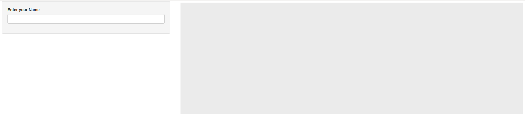
ui <- fluidPage(
textInput('name','Enter your name'),
)
# create server
server <- function(input,output,session){
}
# Run the app
shinyApp(ui,server)
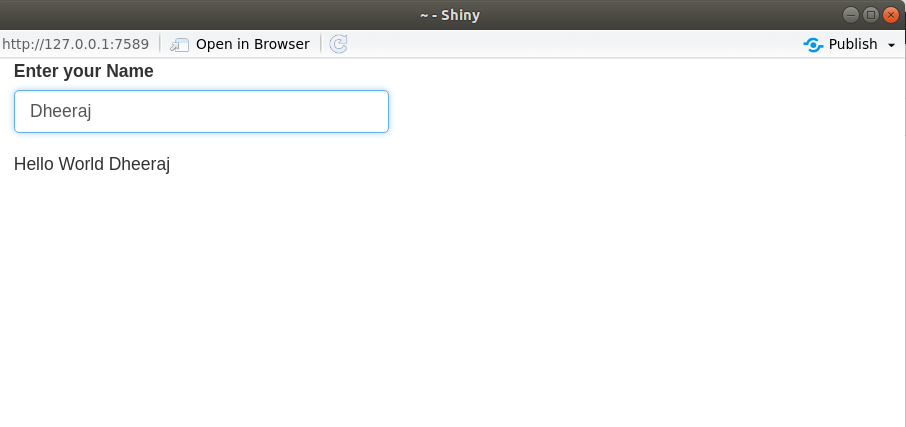
Reactive endpoint
– Something that appears in the user’s browser window, such as a plot or a table of values.
– In simple words, we can say that output that typically appears in the browser window, such as a plot or a table of values.
#load library
library(shiny)
#create ui
ui <- fluidPage(
  textInput('name','Enter your name'),
  textOutput('greeting')

)
#create server
server <- function(input,output,session){
  output$greeting <- renderText({
    paste('Hello ',input$name)
  })

}
#Run the app
shinyApp(ui,server)
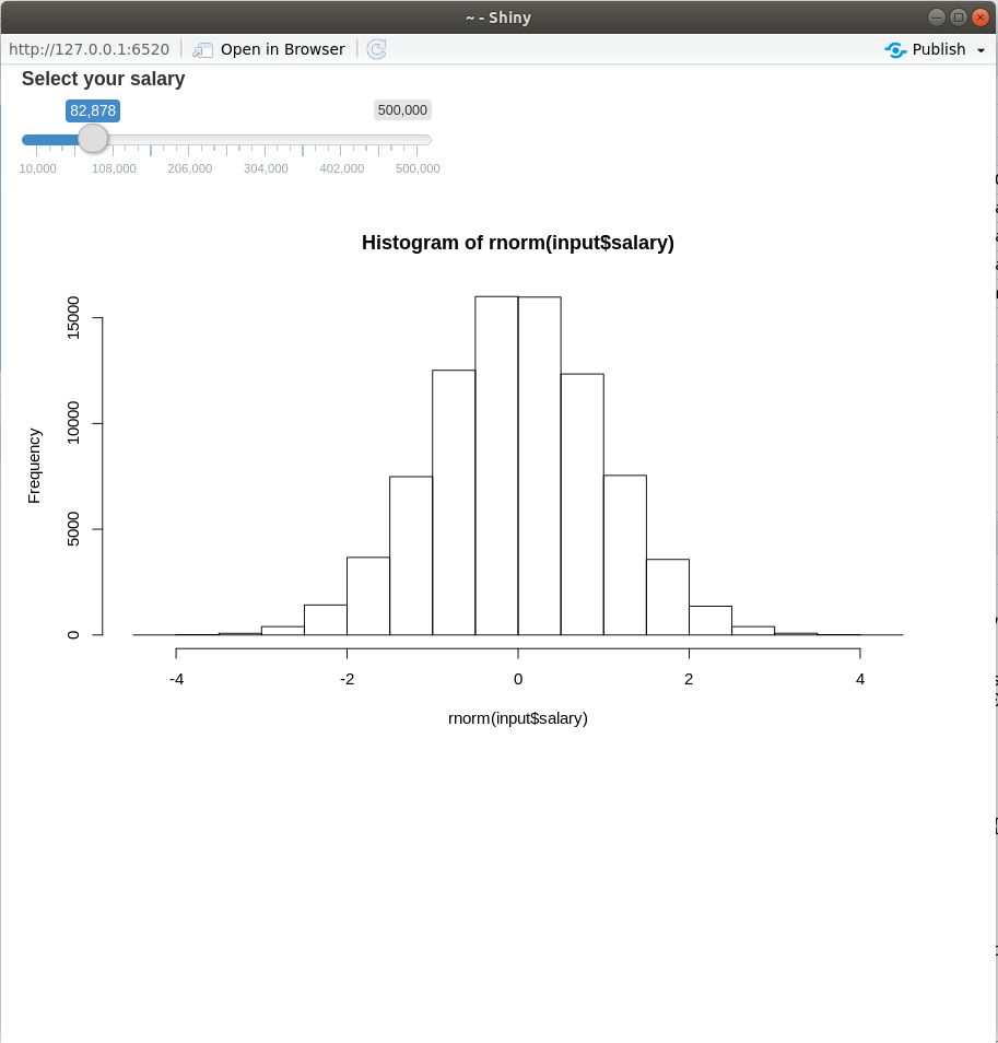
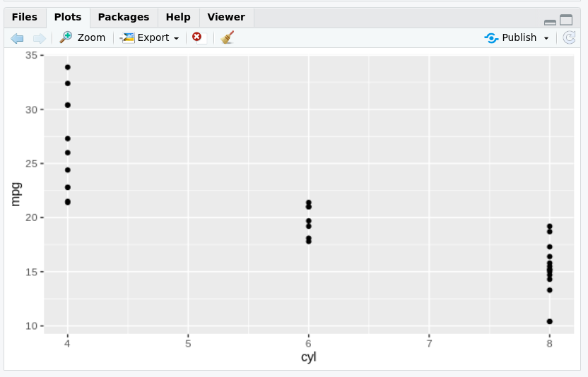
Reactive conductor
– Reactive component between a source and endpoint typically used to encapsulate slow computations.
# create server
server <- function(input,output,session){
  #plot putout
  output$plot_trendy_names <- ploty::renderPlotly({ babynames %>%
      filter(name == input$name) %>%
      ggplot(val_bnames, aes(x=year, y=n)) +
      geom_col()
  })
  #table output
  output$table_trendy_names <- DT::renderDT({ babynames %>%
      filter(name== input$name)
  })
}
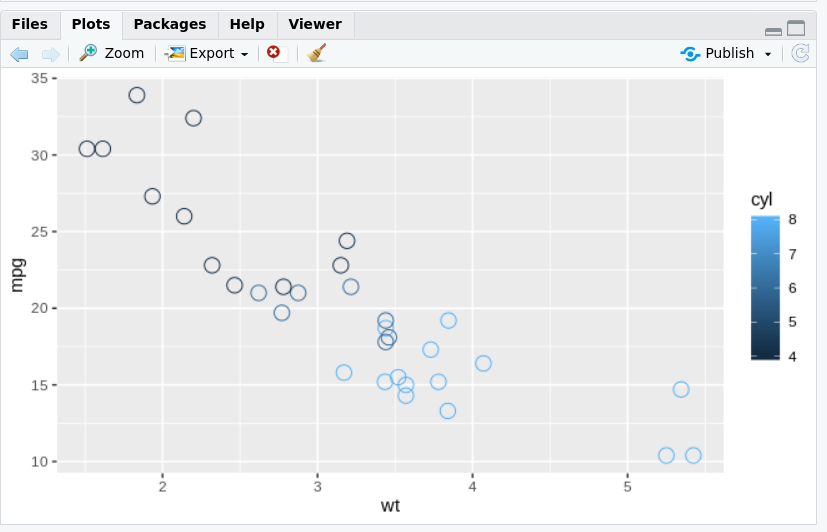
Reactive Expression
– A Reactive expression is an R expression that uses widget input and returns a value.
– The reactive expression will update this value whenever the original widget changes.
– Reactive expressions are lazy and cached.
To create a reactive expression we use reactive function, which takes an R expression surrounded by braces (just like render function).
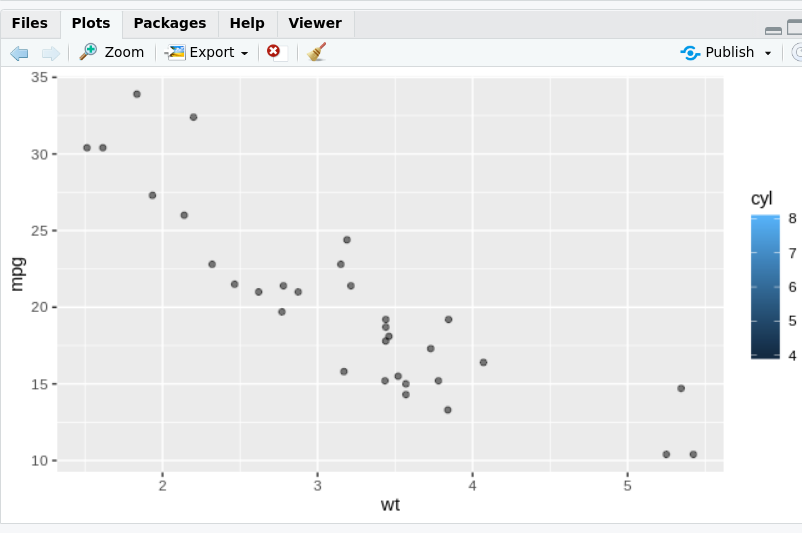
ui <- fluidPage(
  numericInput('nrows', 'Number of Rows', 10, 5, 30),
  tableOutput('table'),
  plotOutput('plot')
)
# create server
server <- function(input, output, session){
 #input 1

  cars_1 <- reactive({
    print("Computing cars_1 ...")
    head(cars, input$nrows)
  })
#input 2
  cars_2 <- reactive({
    print("Computing cars_2 ...")
    head(cars, input$nrows*2)
  })
 #output plot

  output$plot <- renderPlot({
    plot(cars_1())
  })
#output table
  output$table <- renderTable({
    cars_1()
  })
}
# Run the app
shinyApp(ui = ui, server = server)
Note: A reactive expression can call other reactive expressions.That allows us to modularize computations and ensure that they are NOT executed repeatedly.
You should also visit
Build a Hello world shiny App With R