Data visualization Examples in R

In this post, We will explore more examples of Data Visualization using R. For that purpose we are using mtcars as dataset
here is a list of all the features of the observations in mtcars:

  • mpg — Miles/(US) gallon
  • cyl — Number of cylinders
  • disp — Displacement (cu.in.)
  • hp — Gross horsepower
  • drat — Rear axle ratio
  • wt — Weight (lb/1000)
  • qsec — 1/4 mile time
  • vs — V/S engine.
  • am — Transmission (0 = automatic, 1 = manual)
  • gear — Number of forward gears
  • carb — Number of carburetors

Example 1: Plot graph on X and Y axis


# include ggplot2 library
library(ggplot2)

# 1 - Map mpg to x and cyl to y
ggplot(mtcars, aes(x=mpg, y=cyl)) +
  geom_point()

# 2 - Reverse: Map cyl to x and mpg to y
ggplot(mtcars, aes(x=cyl, y=mpg)) +
  geom_point()

OutPut:

Example 2: Change the color, shape, and size of the points


# include ggplot2 library
library(ggplot2)

#chnage color,shape and Size
ggplot(mtcars, aes(x=wt, y=mpg, col=cyl)) +
  geom_point(shape=1, size=4)

OutPut:

Example 3: Add alpha and fill


# include ggplot2 library
library(ggplot2)
# Expand to draw points with alpha 0.5 and fill cyl
ggplot(mtcars, aes(x = wt, y = mpg, fill = cyl)) +geom_point(alpha=0.5)

OutPut:

Exercise 4: Change Shape and color


library(ggplot2)
# Change shape and color
ggplot(mtcars, aes(x = wt, y = mpg, fill = cyl)) +geom_point(shape=24,col="yellow")

OutPut:

Exercise 5: Change shape and Size


# include ggplot2 library
library(ggplot2)
# Define a hexadecimal color
change_color <- "#4ABEFF"
# Set the fill aesthetic; color, size and shape attributes
ggplot(mtcars,aes(x=wt,y=mpg,fill=cyl))+ geom_point(size=10,shape=23,col=change_color)

OutPut:

Explore row data using R

Understanding the structure of your Data

View dimensional

Syntax:


dim()

Example:


# dimensional of mtcars
dim(mtcars)

OutPut:

Looking your DataView dimensional

head()

  • view top of the dataset

Note: By default, it fetches 6 rows but we can also vary a number of rows.
Syntax:


head()

Example:


#head of mtcars
head(mtcars)
# we can vary number of rows
head(mtcars,n=8)

OutPut:

tail()

  • view bottom of the dataset

Example:


#Syntax:tail()
#tail of mtcars
tail(mtcars)

# we can vary number of rows
tail(mtcars,n=8)

Output:
Visualizing your data

hist()

  • view histogram of a single variable

Example:


Syntax:hist()
#histogram
hist(mtcars$mpg)

OutPut:

plot()

  • view plot of two variables

Example:


Synatx: plot()
#plot
plot(mtcars$mpg,mtcars$qsec)

OutPut:

Gather

  • Gather columns into key-value pairs

Syntax:


gather (data, key, value, ...)
/**
 *
data: a data frame
key: bare name of the new key column
value: bare name of the new value column
*/

Spread

  • Opposite of Gather
  • Spread key-value pairs into columns
  • Takes key-value pairs and spread them into multiple columns

Syntax:


spread(data, key, value)
/**
 *
 data: a data frame
 key: bare name of the column containing keys
 value: bare name of the column containing values
*/

Separating columns

  • The separate() function allows you to separate one column into multiple columns.
  • In the case of separate() function, we can also specify sep as an argument for specifying separator.

Syntax:


seperate(data, column_set, c("column1", "column2"))

Uniting column

  • Opposite of separate is unite

Syntax:


unite(data, column-set, c("column1", "column2"))

Note: we can also specify separator between these two columns

Some important functions in R

There are some important functions that we are using in Day to day life. I have categories these functions in these categories for understanding.

  • Common function
  • String Function
  • Looping function

Common function

At first, I am dealing with some common functions in R that we use in day to day life during development.

abs() : Calculate absolute value.

 Example:


  # abs function
  
amount <- 56.50
absolute_amount <- abs(amount)
print(absolute_amount)
sum(): Calculate the sum of all the values in the data structure.

 Example:


  # sum function
  
myList <- c(23,45,56,67)
sumMyList <- sum(myList)
print(sumMyList)
mean() : Calculate arithmetic mean.

 Example:


  # mean function
  
myList <- c(23,45,56,67)
meanMyList <- mean(myList)
print(meanMyList)
round() : Round the values to 0 decimal places by default.

 Example:


  ############## round function #####################
    
  amount <- 50.97
  print(round(amount));
 
seq(): Generate sequences by specifying the from, to, and by arguments.

 Example:

String Function
    
     # seq() function
     # seq.int(from, to, by)
    
  sequence_data <- seq(1,10, by=3)
  print(sequence_data)
  
rep(): Replicate elements of vectors and lists.

 Example:


    #rep exampleString Function
    #rep(x, times)
    sequence_data <- seq(1,10, by=3)  
    repeated_data <- rep(sequence_data,3)
    print(repeated_data)

  
sort(): sort a vector in ascending order, work on numerics.

 Example:


    #sort function
    
  data_set <- c(5,3,11,7,8,1)
  sorted_data <- sort(data_set)Functionround
  print(sorted_data)
  
rev(): Reverse the elements in a data structure for which reversal is defined.

 Example:


   # reverse function 
    String Function
  data_set <- c(5,3,11,7,8,1)
  sorted_data <- sort(data_set)
  reverse_data <- rev(sorted_data)
  print(reverse_data)
  
str(): Display the structure of any R Object.

 Example:


  # str function 
    
  myWeeklyActivity <- data.frame(
    activity=c("mediatation","exercie","blogging","office"),
    hours=c(7,7,30,48)
  )
  print(str(myWeeklyActivity))
  
append() : Merge vectors or lists.

 Example:


   #append function 
    
  activity=c("mediatation","exercie","blogging","office")
  hours=c(7,7,30,48)
  append_data <- append(activity,hours)
  print(append_data)
  
is.*(): check for the class of an R Object.

 Example:


  #is.*() function
    
  list_data <- list(log=TRUE,
                    chStr="hello"
                    int_vec=sort(rep(seq(2,10,by=3),times=2)))
  print(is.list(list_data))
  
as.*(): Convert an R Object from one class to another.

 Example:


  #as.*() function
    
  list_data <- as.list(c(2,4,5))
  print(is.list(list_data))
  

String Function

Now we are discussing some string function that plays a vital role during data cleaning or data manipulation.

These are functions of stringr package.So, before using these functions at first you have to install stringr package.


  # import string library
    
  library(stringr)
 
str_trim () : removing white spaces from string.

 Example:


    ############### str_trim ####################
    
   trim_result <- str_trim(" this is my string test. ");
   print("Trim string")
   print(trim_result)
 
str_detect(): search for a string in a vector.That returns boolean value.

 Example:


  ############### str_detect ####################
    
  friends <- c("Alice","John","Doe")
  string_detect <- str_detect(friends,"John")
  print("String detect ...")
  print(string_detect)
 
str_replace() : replace a string in a vector.

 Example:


  ############## str_replace #####################
    
  str_replace(friends,"Doe","David")
  print("friends list after replacement ....");
  print(friends);
 
tolower() : make all lowercase.

 Example:


  ############## tolower #####################
    
  myupperCasseString <- "THIS IS MY UPPERCASE";
  print("lower case string ...");
  print(tolower(myupperCasseString));
 
toupper() : make all uppercase.

 Example:


  ############## toupper #####################
    
  myupperCasseString <- "My name is Dheeraj";
  print("Upper case string ...");
  print(toupper(myupperCasseString));


Lopping

lapply(): Loop over a list and evaluate a function on each element.

 Some important points regarding lapply :

# lapply takes three arguments:

  1. list X
  2. function (or name the function) FUN
  3. … other argumnts

# lapply always returns list, regardless of the class of input.

Example:


  ############## lapply example #####################
    
  x <- list(a = 1:5,rnorm(10))
  lapply(x,mean)
 

OutPut:

Anonymous function

Anonymous functions are those functions that have no name.


  ############## lapply example #####################
  # Extract first column of matrix 
    
  
  x <- list(a=matrix(1:4,2,2),b=matrix(1:6,3,2))
  lapply(x,function(elt)elt[,1])
 

OutPut:


Use function with lapply


  ############## lapply example #####################
  # multiply each element of list with factor
    
  
  multiply <- function(x,factor){
    x * factor
  }

lapply(list(1,2,3),multiply,factor=3)
 

OutPut:

sapply(): Same as lapply but try to simplify the result.

 Example:


  ############## sapply example #####################
  # multiply each element of list with factor
    
  multiply <- function(x,factor){
    x * factor
  }
sapply(list(1,2,3),multiply,factor=3)
 

OutPut:

apply() : Apply a function over the margin of an array.

 Example:


  ############## apply function #####################
    
  mat1 <- matrix(c(1:10),nrow=5,ncol = 6)
  apply(mat1,2, sum)
 

OutPut:

tapply(): Apply a function over subsets of a vector.

 Example:


  ############## tapply function #####################
    
  tapply(mtcars$mpg, list(mtcars$cyl, mtcars$am), mean)
 

OutPut:

mapply():Multivariate version of lapply.

 Example:

Joins in SQL for Data Analyst

It is the age of Data and now we Data assume data is more precious than Gold. In Data world SQL is one of the best tool used for Data Analysis.

Types of Joins

Basically, there are four types of JOINS in SQL.

      • CROSS JOIN
      • INNER JOIN

                     –   EQUI JOIN
                                 –  NATURAL JOIN

    • OUTER JOIN

                     –   LEFT JOIN (LEFT OUTER JOIN)
                     –   RIGHT JOIN (RIGHT OUTER JOIN)
                     –   FULL JOIN    (FULL OUTER JOIN)

    • SELF JOIN

For practical implementation of JOINS, we are taking two tables 


# Table Details


Products_dataset:-(product_id,product_category_name,product_name_lenght,product_description_lenght,product_photos_qty,product_weight_g,product_length_cm,product_height_cm,product_width_cm)

product_category_name_translation :- (product_category_name	product_category_name_english)

CROSS JOIN

CROSS JOIN returns cartesian product of two tables.

Cartesian Product

If table A contains m rows and table B contains n rows, then cartesian product of table A and table B will contain m*n rows.
Syntax :


# cross join syntax


SELECT * FROM tableA CROSS JOIN tableB

     or
     
SELECT * FROM tableA,tableB

Example :


SELECT * FROM products_dataset CROSS JOIN product_category_name_translation

OutPut:

INNER JOIN

return all rows from tableA where there are matching values in tableB and all columns from tableA and tableB. If there are multiple matches between tableA and tableB then all matches will return from tableA and tableB on the basis of a specified condition.

And condition has been mentioned in the syntax after the last table.
Syntax:


# Inner join syntax

SELECT * FROM tableA INNER JOIN tableB ON (tableA.x = tableB.y)


or 

SELECT * FROM tableA JOIN tableB ON (tableA.x = tableB.y)

Note: By default, JOIN is considered as INNER JOIN or EQUI JOIN.

Example :


# inner join example

SELECT * FROM products_dataset pds INNER JOIN product_category_name_translation pct
ON pds.product_category_name=pct.product_category_name

OutPut :

LEFT JOIN (LEFT OUTER JOIN) :

return all rows from tableA, and all columns from tableA and tableB. Rows in tableA with no match in tableB will have NA values in the new columns. If there are multiple matches between tableA and tableB, all combinations of the matches are returned.
Syntax :


# left join syntax

SELECT * FROM tableA LEFT JOIN tableB ON (tableA.x = tableB.y)

Example:


#  left join example

SELECT * FROM products_dataset pds LEFT JOIN product_category_name_translation pct

ON pds.product_category_name=pct.product_category_name

OutPut :

RIGHT JOIN (RIGHT OUTER JOIN)

return all rows from tableB, and all columns from tableA and tableB. Rows in tableB with no match in tableA will have NA values in the new columns. If there are multiple matches between tableA and tableB, all combinations of the matches are returned.
Syntax:


# right join syntax

SELECT * FROM tableA RIGHT JOIN tableB ON (tableA.x = tableB.y)

Example:


#  right join example

SELECT * FROM products_dataset pds RIGHT JOIN product_category_name_translation pct
ON pds.product_category_name=pct.product_category_name

OutPut:

Joining data in R using Dplyr

Working with data, Joining is the common operation.

Joining means combine i.e combine the data from two or more than two different sources on the basis of some conditions.

For performing such type of operation in R dplyr is the best option for doing so.

During this post, we will these key points.

  • Types of Joins in R
  • Syntax
  • Joining on DataFrame
  • Joining on tables

Types of Joins

There are six types of Joins in R :

  1. Inner Join (inner_join)
  2. Left Join (left_join)
  3. Right Join (right_join)
  4. Full Join (full_join)
  5. Semi Join (semi_join)
  6. Anti Join (anti_join)

Syntax


# Syntax of Joining in R

Join_type(x,y,by=condition)

/**
  * x: dataframe1/table1
  * y: dataframe2/table2
*/

Joins are basically applied on tables and in case of R files are to be considered as tables.

For a better understanding of joins, we are taking two files 

  1. Product_category_name.csv (product_category_name, product_category_name_english)
  2. product_dataset.csv(product_id,product_category_name,product_name_lenght, product_description_lenght, product_photos_qty, product_weight_g, product_length_cm, product_height_cm, product_width_cm)

You can download these files for your practice my GitHub account

As we know during applying joins on two different datasets or tables we need a common field on the basis of that we can be able to apply a join.

So, in this case, both files contain product_category_name so on the basis of that we can apply to join.

For using a CSV file as a table we are using command 


# read csv file

read.csv(file_name)

So for applying joins on these two files at first, we have to consider these two files as two tables using read.csv() command. As shown below.


# load data


table1 <- read.csv("/home/dheeraj/Desktop/Blog_post/joins_in_r_using_dplyr/dataset/product_category_name.csv") # file location of Product_category_name.csv
table2 <- read.csv("/home/dheeraj/Desktop/Blog_post/joins_in_r_using_dplyr/dataset/products_dataset.csv")   # file location of product_dataset.csv 

Inner Joins

Syntax :


# inner join syntax


inner_join(x,y,by='condition')

Examples :

Select all columns

library(dplyr)
table1 <- read.csv("/home/dheeraj/Desktop/Blog_post/joins_in_r_using_dplyr/dataset/product_category_name.csv") # file location of Product_category_name.csv
table2 <- read.csv("/home/dheeraj/Desktop/Blog_post/joins_in_r_using_dplyr/dataset/products_dataset.csv")   # file location of product_dataset.csv 

appliedInnerJoin <- inner_join(table1,table2,by='product_category_name')

print(head(appliedInnerJoin,n =20))

OutPut:

Select specified columns

If we don’t want to extract all columns then we can select specified columns using select command.

Suppose In this after applying inner join on table1 and table2 we don’t want to extract all columns of these tables but also we want to extract only
product_id.product_category_name_english.

Then we can use select command of dplyr package (for more detail click here) and extract specified columns that we want to extract

Example


library(dplyr)
table1 <- read.csv("/home/dheeraj/Desktop/Blog_post/joins_in_r_using_dplyr/dataset/product_category_name.csv") # file location of Product_category_name.csv
table2 <- read.csv("/home/dheeraj/Desktop/Blog_post/joins_in_r_using_dplyr/dataset/products_dataset.csv")   # file location of product_dataset.csv 

appliedInnerJoin <- inner_join(table1,table2,by='product_category_name')
#select specified column

specified_columns <- select(appliedInnerJoin,product_id,product_category_name_english)
print(specified_columns)

OutPut:

left join

Syntax :


left_join(x,y,by='condition')
 

Example:


library(dplyr)
table1 <- read.csv("/home/dheeraj/Desktop/Blog_post/joins_in_r_using_dplyr/dataset/product_category_name.csv") # file location of Product_category_name.csv
table2 <- read.csv("/home/dheeraj/Desktop/Blog_post/joins_in_r_using_dplyr/dataset/products_dataset.csv")   # file location of product_dataset.csv 
# left join
appliedLeftJoin <- left_join(table1,table2,by='product_category_name')<img src="http://www.krdheeraj.info/wp-content/uploads/2020/01/leftJoin.png" alt="" width="1345" height="579" class="alignnone size-full wp-image-496" />

print(head(appliedLeftJoin,n=10))

OutPut:

right join

Syntax :


right_join(x,y,by='condition')
 

EXample


library(dplyr)
table1 <- read.csv("/home/dheeraj/Desktop/Blog_post/joins_in_r_using_dplyr/dataset/product_category_name.csv") # file location of Product_category_name.csv
table2 <- read.csv("/home/dheeraj/Desktop/Blog_post/joins_in_r_using_dplyr/dataset/products_dataset.csv")   # file location of product_dataset.csv 
# left join
appliedRightJoin <- right_join(table1,table2,by='product_category_name')

print(head(appliedRightJoin,n=10))

Output:

Dplyr grammar of Data Manipulation in R

dplyr package is used for Data Manipulation in R.

So it is the reason that’s why dplyr is called grammar of Data Manipulation.

With the help of dplyr package, we can be able to manipulate data and extract useful information easily and quickly.

Installing and loading dplyr package in R

Installing dplyr


/**
  * install dplyr package
*/

install.package("dplyr")

loading dplyr


/**
  * load dplyr package
*/

library(dplyr)

dplyr package contains 5 verbs for Data Manipulation. That we will discuss in this post.

dplyr 5 verbs for Data Manipulation

Dplyr Function Description
Select () Returns subset of the Columns.
Filter() Returns subset of Rows.
Arrange() Reorder rows according to single or multiple variables.
Mutate() Used for adding a new column from the existing column.
Summarize() Reduce each group to a single row by calculate aggregate measure.

For Exploring our knowledge in dplyr we have need a dataset.

So for that purpose, I am loading a variable.

For reading a CSV file we are using read.csv function.

Syntax :


/**
  * load dplyr package
*/


read.csv("file location")

Example:


/**
  * load dplyr package
*/

load_csv_data <- read.csv("/home/dheeraj/Downloads/brazilian-ecommerce/order_items_dataset.csv") ///

print(load_csv_data)

OutPut:

read csv file
Although read.csv() always return data.frame.

We can be able to store read.csv() return inside a variable as in previous example we are storing in load_csv_data. So if we are accessing variable it means we are accessing that data.

Now we are performing some operation with dplyr Package.
For that purpose, we taking all functions of dplyr package and performing some operations.

But Before using dplyr 5 verbs. We should observe our data on which we are going to implement dplyr verbs.
And dplyr package contains a separate function glimpse() for that purpose.


glimpse(): returns Observation of Data frame.
Syntax :


/**
  * load dplyr package
*/

glimpse(data_frame)

Example:


/**
  * load dplyr package
*/

glimpse(load_csv_data)

OutPut:
glimpse
So glimpse() function provides details about our dataframe.
Now we understood that our data frame contains 112,650 rows and 7 columns as shown below.


Observations: 112,650
Variables: 7
$ order_id            
$ order_item_id       
$ product_id          
$ seller_id          
$ shipping_limit_date 
$ price               
$ freight_value

Selecting Column using Select

Select returns subset of columns.
In other words, we can also say that remove columns from the dataset.
Syntax :


/**
  * select syntax
*/

Select(df, column1,column2)
Where df: data frame 
      Column1: name of column1
      Column2: name of column2

Example:

We have already loaded our data inside our load_csv_data variable. So Now perform these following actions

  • Extract order_id,product_id,price from load_csv_data.
  • Extract order_id,order_item_id, product_id,seller_id,shipping_limit_date,price from load_csv_data.
  1. Extract order_id,product_id,price from load_csv_data.


/**
  * select example for extracting columns 
*/

select_Columns <- select(load_csv_data,order_id,product_id,price)

print(select_Columns)

OutPut:

2. Extract order_id,order_item_id, product_id,seller_id,shipping_limit_date,price from load_csv_data.


/**
  * select example for extracting columns 
*/

select_Columns <- select(load_csv_data,order_id,order_item_id, product_id,seller_id,shipping_limit_date,price)

print(select_Columns)

OutPut:

If we have to access columns in a sequence i.e no column should be removed from the sequence.

As in the previous example, we want to access from order_id to price and these columns are in sequence and no column is missing inside sequence.

In this case, we can access our columns like 


/**
  * syntax for select verb in dplyr 
*/


select(data_frame,column1:column(N-i))

So we can also perform our previous operation in this way.


/**
  * select example for extracting columns 
*/


select_Columns <- select(load_csv_data,order_id:price)

print(select_Columns)

OutPut:

Select rows using filter

glimpse() is used for filtering rows on basis of condition.
Syntax:


/**
  * filter syntax
*/

filter(data_frame,condition1 ... condition(N-i))

Example:

Filter row on basis of single condition

Extract row from load_csv_data data frame of which order_id is 5.


/**
  * filter example
*/


selected_rows <- filter(load_csv_data,order_id==5)

print(selected_rows)

OutPut:

Filter row on the basis of multiple conditions.

Extract rows from load_csv_data from which order_item_id=1 and shipping_limit_date= 2017-11-27 19:09:02


/**
  * filter example
*/
 

selected_rows_multiple_conditions <- filter(load_csv_data,order_item_id==1,shipping_limit_date==	 '2017-11-27 19:09:02')

print(selected_rows_multiple_conditions)

OutPut:

Import CSV file in MySQL database using SQL


During Data Analysis it is a common situation during which we have to import CSV files into MYSQL database.

In this post, we will discuss the same scenario and a simple way for importing CSV files using SQL.

Before importing a CSV file we need to create a table that will contain all columns of CSV file.

Suppose I have CSV file order_items_dataset.csv and we want to import this CSV file in  MYSQL Database.

import csv file


Then before importing CSV file, we have to create a table in MYSQL Database.

So, At first, we are creating a table

Create a table in MYSQL Database


/**
  * create order_items_datasets table for importing csv file
*/

CREATE TABLE order_items_datasets (
order_id int PRIMARY KEY,
order_item_id int,
product_id varchar (200),
seller_id varchar(200),
shipping_limit_date DATETIME,
price float,
freight_value float
)

Now our table has been created successfully.

Now we need to import CSV file in order_items_datasets table.

For that, we have to follow these few steps.

STEP 1:   Load Data

For that purpose, we will LOAD DATA Statement.

LOAD DATA Statement: reads a row from a text file into a table with a very high speed.  


# comment line

LOAD DATA

Step 2: Include CSV file

For including CSV file from which we have to import Data we used INFILE command with LOAD DATA  Statement.

INFILE: allow us to read CSV data from a text file.

NOTE: LOAD DATA INFILE statement allows us to read CSV data from a text file and import that into a database table with very fast speed.  

So for Including a file, we will write 


# comment line

LOAD DATA INFILE "/home/dheeraj/Downloads/brazilian-ecommerce/order_items_dataset.csv"  -- file location

Step 4: Import Data to table

For importing data inside the table we will add INTO then after table name with LOAD DATA statement. 

As shown below for importing data into my new table order_items_datasets that we have created previously.


# import data inside table


LOAD DATA INFILE "/home/dheeraj/Downloads/brazilian-ecommerce/order_items_dataset.csv" -- file location
INTO TABLE order_items_datasets -- table name 

Step4: Extract values from CSV file 

CSV file contains comma-separated values. So we need to separate these values on the basis of rows and columns.

For this, we will add these few lines


# comment line

FIELDS TERMINATED BY ',' 
ENCLOSED BY '"'
LINES TERMINATED BY '\n'

Step5: Ignore header of CSV file

During importing CSV file we need to ignore the header. For this, we will add this line.


# ignore header 

IGNORE 1 ROWS;

After following these steps we can be able to import CSV files in MYSQL database.

Complete Query:


/**
Create table
*/

CREATE TABLE order_items_datasets (
order_id int PRIMARY KEY,
order_item_id int,
product_id varchar (200),
seller_id varchar(200),
shipping_limit_date DATETIME,
price float,
freight_value float
)

--  load data 
LOAD DATA

-- include file

LOAD DATA INFILE "/home/dheeraj/Downloads/brazilian-ecommerce/order_items_dataset.csv"  -- file location

-- import data inside table

LOAD DATA INFILE "/home/dheeraj/Downloads/brazilian-ecommerce/order_items_dataset.csv" -- file location
INTO TABLE order_items_datasets -- table name 

-- extract data

FIELDS TERMINATED BY ',' 
ENCLOSED BY '"'
LINES TERMINATED BY '\n'

-- ignore header

IGNORE 1 ROWS;

Basic Of SQL for Data Analysis

Introduction to SQL :

SQL stands for Structural Query Language. 

According to the survey of StackOverflow SQL always remains in the top 5 programming language in the world.

It means you are learning one of the most popular language in the world.

Operation in SQL :

Create Operation :

Create Operation is most basic operation in SQL. 

Create operation is used for multiple purposes like creating a table, creating schema, etc.

For performing a Create Operation, we use Create Command with some keyword as

CREATE SCHEMA :

CREATE SCHEMA command is used for creating schema in SQL

Syntax:


/**
CREATE SCHEMA 
*/

CREATE SCHEMA shema_name;

Example: 


/**
CREATE SCHEMA 
*/

CREATE SCHEMA e_commerce_db;

CREATE TABLE :

Used for Creating table
Syntax :


/**
CREATE SCHEMA 
*/

CREATE TABLE table_name (column_name1 data type  key order_detailsconstraints,column_name1 data type  key constraints … column_namen data type  key constraints)

Example:


/**
CREATE TABLE 
*/
Create table professionals_records(
id int primary key not null AUTO_INCREMENT,
name varchar (100),
mobile varchar(10),
email varchar(200),
city varchar(100),
occupation varchar(200),
designation varchar(100),
salary float
)

CREATE VIEW :

After creating table SELECT command is used for view data inside table (latter discussed about SELECT command). But in the case of SQL, we don’t show the same data for all users. So, in that case, we have to CREATE VIEW.

Syntax :


/**
CREATE SCHEMA 
*/

CREATE VIEW AS view_name( Query for view) 

Note: We will explain the Example of View latter in the same post.

shown below in the table

Create Operation Summary

Create command with keyword Description Syntax Example
CREATE SCHEMA For creating Schema in Database CREATE SCHEMA schema_name CREATE SCHEMA e_commerce_db
CREATE TABLE For creating table in Database CREATE TABLE table_name(column_name data type key constraints , …) CREATE TABLE order_details(id int primary key, name varchar(25) )
CREATE VIEW Used for Creating a view in Database CREATE VIEW AS view_name (query for creating a view) CREATE VIEW AS view_name(SELECT name FROM order_details)
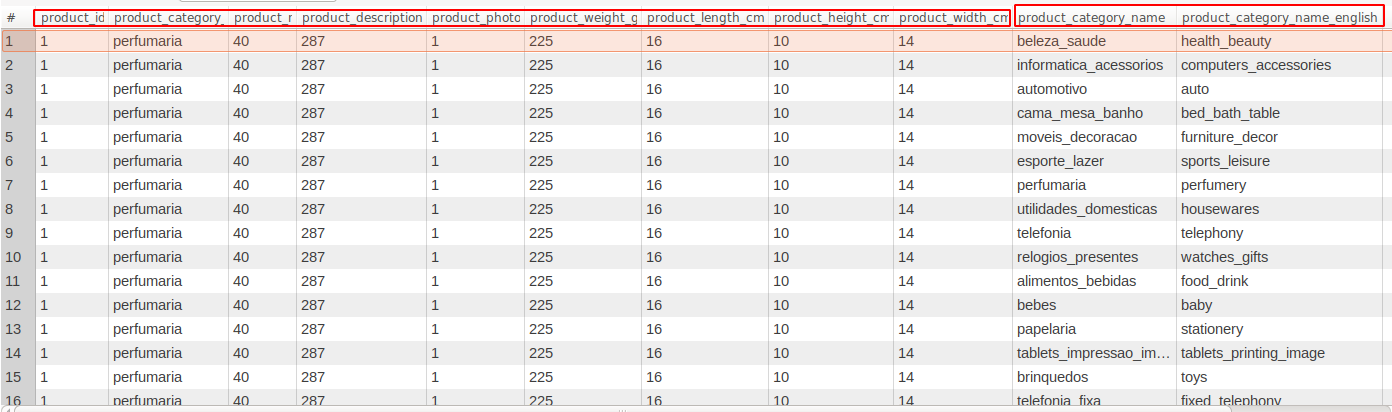
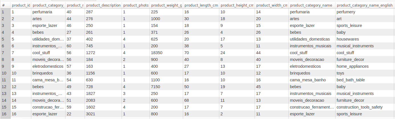
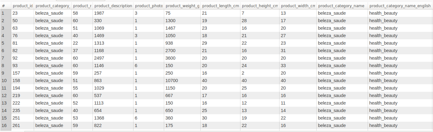
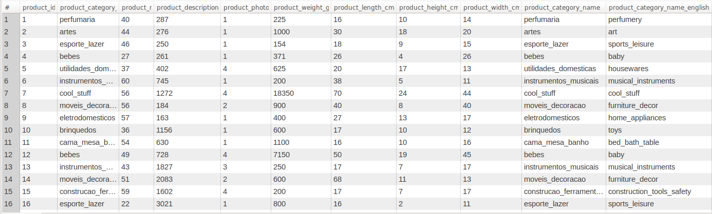
order_details

Insert Operation

For Inserting rows inside a table we use insert command.
There are two different ways for Inserting rows inside the table :

  1. order_detailsInserting a single row inside a table
  2. Inserting multiple rows inside a table

Inserting a single row inside a table :

Syntax:


# comment line

INSERT INTO TABLE table_name(column1,column2,column3 ... , columnN) VALUES(value1,value2,value3 ..., valueN)

Example:

order_details

# Insert Single line


INSERT INTO professionals_records (id,name,mobile,email,city,occupation,designation,salary) 
values (1,'Nitin verma','7739042930','nverma@gmail.com','Jaipur','Engineer','Manager',100000)

Inserting multiple rows inside a table :

Syntax:

order_details

# comment line

INSERT INTO TABLE table_name(column1,column2,column3 ... , columnN) 
VALUES(value1,value2,value3 ..., valueN),
(value1,value2,value3 ..., valueN),
(value1,value2,value3 ..., valueN)
 .
 .
 . 
(value1,value2,value3 ..., valueN)

Example


# Insert Multiple lines


INSERT INTO professionals_records (id,name,mobile,email,city,occupation,designation,salary) 
values 
(1,'Nitin Verma,'7739042930','nverma@gmail.com','Jaipur','Engineer','Manager',100000),
(2,'Mukesh Sharma','9939042932','msharma@gmail.com','Jaipur','Engineer','Software Developer',50000),
(3,'Nimesh Mehra','8965721230','rmehra@gmail.com','Jaipur','Engineer','Software Developer',60000)order_details

SELECT Operation:

SELECT Statement return result set of records from one or more tables.
Syntax:


# comment line

SELECT * FROM table_name 

Note : * denotes all column

Example:


# Select query
SELECT * FROM professionals_records 

we can also specify specific columns also for extracting a particular column.
Syntax:


# comment line

SELECT column1, column2 ... columnN FROM table_name

Example:


# Select query

SELECT name,mobile,email,city,occupation FROM professionals_records; 

WHERE clause :

It is the most important keyword for SELECT Operation.
It is basically used for filtering data from SQL tables.
Syntax:


# comment line

SELECT * FROM table_name WHERE 

Example :


# comment line

SELECT * FROM professionals_records WHERE id=3;

Note: WHERE clause is not only used SELECT statement but also it is also used with UPDATE, DELETE statement.

LIMIT keyword

It is used for limiting how many number of rows that we want to extract.

Syntax :


# comment line

LIMIT number_of_rows;

Example:


order_details
# comment line

SELECT * FROM professionals_records LIMIT 2;

In the above example it will extract only 2 rows from professionals_records table.

Aggregate Function :

Aggregate function basically used for apply a calculation on a column.
It is also used for filtering some value on the basis of some calculations.

Types of Aggregate Function

  • AVG
  • SUM
  • COUNT
  • MIN
  • MAX

Note: AVG, SUM, MIN are applied to numerical values. So before applying these functions on a particular column make sure that the column contains numerical values or not.

Aggregate Function Description Example
AVG() Calculate average of a particular column SELECT avg(salary) FROM professionals_records;
SUM() Calculate sum of selected column SELECT sum(salary) FROM professionals_records;
COUNT() Count number of records (rows) SELECT count (*) FROM professionals_records;order_details
MIN() Return minimum value on applied column SELECT MIN(salary) FROM professionals_records;
MAX() Return maximum value of applied column SELECT MAX(salary) FROM professionals_records;

UPDATE Operation:

Used for updating records inside table.
For changing rows data inside a table we use UPDATE command.order_details
Syntax :


# comment line

UPDATE TABLE table_name set column_name=;

Example :


# comment line


UPDATE TABLE professionals_records SET salary=25000

Just wait from the above query all the values of the salary of all employees will be interchanged with 25000.
And we obviously don’t want to do so.

How do we avoid making such type of mistake?

For avoiding such types of mistakes, we will use WHERE Clause.
Syntax:


# comment line

UPDATE TABLE table_name SET column_name= WHERE ;

Example:


order_details
# comment line


UPDATE TABLE professionals_records SET salary=25000 WHERE id=1

Above query update salary=25000 of which id is 1.

DELETION Operation :

order_detailsDeletion Operation is done for deleting records from Database.
For deleting records from the Database table we use Delete Statement.
Syntax:


# comment line

DELETE TABLE table_name 

Example:

order_details

# comment line

DELETE TABLE professionals_records

It will delete all records from the professionals_records table.
For deleting particular records, we will have to use WHERE clause as shown below.

DELETE Statement with WHERE Clause

order_detailsorder_detailsSyntax :


# comment line

DELETE TABLE table_name WHERE  

Example:


# comment line


DELETE TABLE professionals_records WHERE id=25;

Delete records only for which id is 25.

Introduction to Puppeteer

Puppeteer is a Node.js library that allows you to control Chrome browser from JS code. Most things that you can do manually in the browser can be done using Puppeteer. Here are a few examples to get you started:

Most things that we do manually in the browser.Can be done using puppeteer easily.

What we can do?

  • Scrap web page
  • Automate process on the web
  • Take screenshot of web pages
  • Generate pdf from HTML

How to start with Puppeteer?

For starting with Puppeteer we have to follow these few steps

    1. Install Puppeteer
    2. Load Puppeteer module
    3. Launch Browser
    4. Headless mode
    5. Open tab inside Browser
    6. Open page inside Browser
    7. Close Browser

Install Puppeteer


Installing Puppeteer

Load Puppeteer package

In node.js we load the package using require like


const puppeteer = require('puppeteer');

Launch browser

To launch browser with puppeteer we have to use launch() method


(async () => {
 const browser = await puppeteer.launch();
})();

We can also write this


puppeteer.launch().then(async browser =>{
});

Headless mode

Puppeteer launches chromium in headless mode.

By default puppeteer launch in headless mode i.e


{headless:true}

This means when we will run the application our browser will not be opened.
But during the process, we can make our browser open and for this, we have to make

Open tab inside Browser

nextPage() method on browser object to get page Object.


const puppeteer = require('puppeteer');

(async () => {

const browser=await puppeteer.launch();
const page=await browser.newPage();
});

Open page inside Browser

page.goto() method used for open particular page inside opened browser


const puppeteer = require('puppeteer');

(async () => {

const browser=await puppeteer.launch();
const page=await browser.newPage();
await page.goto("https://google.com/");
});

Close Browser

Textbrowser.close() Used for close browser Once task has been completed.


await browser.close(); 

Example :

Here we are opening google.com using puppeteer


const puppeteer = require('puppeteer');

(async () => {
 const browser = await puppeteer.launch();
 const page = await browser.newPage();
 await page.goto('https://google.com/');
 await browser.close();
})();

For running application we use command
During the above process, the browser will be opened and closed and we can’t be able to track the process. Because in this case {headelss: true}

If we want to track process then, in that case, we have to take {headelss: false}. In this case, the browser will be visualized and we can be able to see steps and debug our code if required.


const puppeteer = require('puppeteer');

const puppeteer = require('puppeteer');

(async () => {
 const browser = await puppeteer.launch({headless:false});
 const page = await browser.newPage();
 await page.goto('https://google.com/');
 await browser.close();
})();

Here we are not dealing with all methods of puppeteer because it has been already done on its official site https://pptr.dev/.

What are we doing here?

Our main purpose is to take an idea of puppeteer and making projects so that we have a good hand on puppeteer.
For this purpose, we need to familiar with some important classes and modules of puppeteer and that we will cover here.

Classes of puppeteer module

These are some important classes of puppeteer module

page method

page class is a very important class in the puppeteer module. Without creating page Object we can’t be able to open a page on chrome browser.

Some methods of page() class

Method Way to write Description
$(selector) await page.$(‘.common’) querySelector on the page.
$$(selector) await page.$$(‘#intro’) querySelectorAll on the page.
goto(url) await page.goto(‘url’) a
Used for open a specified url.
content() await page.content() Get an HTML source of the page.
click(selector) await page.click(‘button#submit’) a
Mouse click event on the element pass as a parameter.
hover(selector) await page.hover(‘input[name=”user”]’) Hover particular elemet.
reload() await page.reload() a
Reload a page.
pdf() await page.pdf({path:’file.pdf’}) Generate pdf for open url page.
screenshot() await page.screenshot({path:file.png’}) Take screenshot of page and save as png format.

Web Scraping with R

Now a days to run a business we have need to understand business pattern, Client behavior, Culture, location, environment. In the absence of these, we can’t be able to run a business successfully.

With the help of these factors, the probability of growing our business will become high.

So, In simple terms to understand and run a business successfully, we have need Data from which we can be able to understand Client behavior, business pattern, culture, location, and environment.

Today one of the best sources for collecting data is web and to collect data from the web there are various methods.

One of them is Web Scraping in different languages we extract data from web from different ways.

Here we will discuss some of the methods for extracting data from the web using R Language.

There are various resources on the web and we have various techniques for extracting data from these different resources.

Some of these resources are :

    • Google sheets
    • Wikipedia
    • Extracting Data from web tables
    • Accessing Data from Web 

Read Data in html tables using R

Generally for storing large amounts of data on the web, we use tables and here we are discussing the way for extracting data from html tables. So, without further delay, we are following steps for extracting data from html tables.

During this session, we have design some steps  so that anyone can be able to access html tables following steps:

  1. Install library
  2. Load library
  3. Get Data from url
  4. Read HTML Table
  5. Print Result

Install library


# install library
install.packages('XML')
install.packages('RCurl')

During reading data from web generally, we used these library 


# load library 
library(XML)
library(RCurl)

Get Data from url

During this session, we will extract the list of Nobel laureates from Wikipedia page and for that at first copy url of table and here is url


https://en.wikipedia.org/wiki/List_of_Nobel_laureates#List_of_laureate

In R we write these lines of code for getting data from url.


# Get Data from url
url <- "https://en.wikipedia.org/wiki/List_of_Nobel_laureates#List_of_laureates"
url_data <- getURL(url)

Read HTML Table

Now it’s time to read table and extract information from the table and for that we will use readHTMLTable() function.


# Read HTML Table
data <- readHTMLTable(url_data,stringAsFactors=FALSE)

Print Result

Finally, our data has been stored in data variable and now we can print this


# print result
print(data) 

Here is complete code for reading HTML table from web using R


# install library
install.packages('XML')
install.packages('RCurl')
# load library 
library(XML)
library(RCurl)
# Get Data from url
url <- "https://en.wikipedia.org/wiki/List_of_Nobel_laureates#List_of_laureates"
url_data <- getURL(url)
# Read HTML Table
data <- readHTMLTable(url_data,stringAsFactors=FALSE)
# print result
print(data)

rvest package for Scraping

rvest is most important package for scraping webpages. It is designed to work with magrittr to make it easy to scrape information from the Web inspired by beautiful soup.

Why we need some other package when we already have packages like XML and RCurl package?

During Scraping through XML and RCurl package we need id, name, class attribute of that particular element.
If Our element doesn’t contain such type of attribute, then we can’t be able to Scrap information from the website.
Apart from that rvest package contains some essential functions that enhance its importance from other packages.
During this session also, we have to follow the same steps as we have designed for XML and RCurl package access HTML tables. We are repeating these steps :

    1. Install package
    2. Load package
    3. Get Data from url 
    4. Read HTML Table
    5. Print Result

we are repeating same example as we have discussed before but with rvest package.

Install package


# install package
install.packages('rvest')

Load package


#load package
library('rvest')

Get Data from url and Read HTML Table


url <- 'https://en.wikipedia.org/wiki/List_of_Nobel_laureates'
# Get Data from url and Read HTML Table 
prize_data <- url %>% read_html() %>% html_nodes(xpath = '//*[@id="mw-content-text"]/div/table[1]') %>%
  html_table(fill = TRUE)

Here we have combined two steps with a single step and i.e beauty of piping in R. Apart from that inside html_nodes() method we have used XPath.
Yeah with rvest package we have to use Xpath of element that we want to copy.
And steps for copy XPath as shown below inside image in which we are copying XPath of table

print Data


#print Data
print(prize_data)

Here is complete code for reading HTML table from web using rvest in R


# install package

install.packages('rvest')

#load package
library('rvest')
url <- 'https://en.wikipedia.org/wiki/List_of_Nobel_laureates'
# Get Data from url and Read HTML Table
prize_data <- url %>% read_html() %>% html_nodes(xpath = '//*[@id="mw-content-text"]/div/table[1]') %>%
  html_table(fill = TRUE)
# read prize data
print(prize_data)

Both example i.e reading table with XML and RCurl package and reading the same table with rvest package that will be looked like 
Output:

web Scraping output in R
Note : we will go through more examples on rvest in the next post but before that we took a quick introduction of googlesheets package in R.

Extracting Data from Google sheets :

Google sheets became one of the most important tools for storing data on the web. It is also useful for Data Analysis on the web.

In R we have a separate package for  extracting Data from web i.e googlesheets

How to use Google Sheets with R?

In this section, we will explain how to use googlesheets package for extracting information from google sheets.

We have the process of extracting data from google sheets  in 5 steps

  1. Installing googlesheets 
  2. Loading googlesheets 
  3. Authenticate google account
  4. Show list of worksheets
  5. Read a spreadsheets
  6. Modify the sheet

Install googlesheets package


install.package("googlesheets")

Loading googlesheet


library("googlesheets")

Authenticate google account


gs_ls()

After that in the browser authentication page will be opened like shown below

Complete code


 # install packages 
 install.packages('googlesheets') 
 # load library
 library('googlesheets')
 # Authentication complete,Please close this page and return 
 gs_ls()
 # take worksheet with title
 take_tile <- gs_title("amazon cell phone items")
 #get list of worksheets
  gs_ws_ls(be)
    

More Tutorials on R

Introduction to Text mining in R

Introduction to Text mining in R Part 2

Create Word Cloud in R