There are some important functions that we are using in Day to day life. I have categories these functions in these categories for understanding.
- Common function
- String Function
- Looping function
Common function
At first, I am dealing with some common functions in R that we use in day to day life during development.
abs() : Calculate absolute value.
Example:
  # abs function

amount <- 56.50
absolute_amount <- abs(amount)
print(absolute_amount)
sum(): Calculate the sum of all the values in the data structure.
Example:
  # sum function

myList <- c(23,45,56,67)
sumMyList <- sum(myList)
print(sumMyList)
mean() : Calculate arithmetic mean.
Example:
  # mean function

myList <- c(23,45,56,67)
meanMyList <- mean(myList)
print(meanMyList)
round() : Round the values to 0 decimal places by default.
Example:
  ############## round function #####################

  amount <- 50.97
  print(round(amount));
seq(): Generate sequences by specifying the from, to, and by arguments.
Example:
String Function

     # seq() function
     # seq.int(from, to, by)

  sequence_data <- seq(1,10, by=3)
  print(sequence_data)
rep(): Replicate elements of vectors and lists.
Example:
    #rep exampleString Function
    #rep(x, times)
    sequence_data <- seq(1,10, by=3)
    repeated_data <- rep(sequence_data,3)
    print(repeated_data)
sort(): sort a vector in ascending order, work on numerics.
Example:
    #sort function

  data_set <- c(5,3,11,7,8,1)
  sorted_data <- sort(data_set)Functionround
  print(sorted_data)
rev(): Reverse the elements in a data structure for which reversal is defined.
Example:
   # reverse function
    String Function
  data_set <- c(5,3,11,7,8,1)
  sorted_data <- sort(data_set)
  reverse_data <- rev(sorted_data)
  print(reverse_data)
str(): Display the structure of any R Object.
Example:
  # str function

  myWeeklyActivity <- data.frame(
    activity=c("mediatation","exercie","blogging","office"),
    hours=c(7,7,30,48)
  )
  print(str(myWeeklyActivity))
append() : Merge vectors or lists.
Example:
   #append function

  activity=c("mediatation","exercie","blogging","office")
  hours=c(7,7,30,48)
  append_data <- append(activity,hours)
  print(append_data)
is.*(): check for the class of an R Object.
Example:
  #is.*() function

  list_data <- list(log=TRUE,
                    chStr="hello"
                    int_vec=sort(rep(seq(2,10,by=3),times=2)))
  print(is.list(list_data))
as.*(): Convert an R Object from one class to another.
Example:
  #as.*() function

  list_data <- as.list(c(2,4,5))
  print(is.list(list_data))
String Function
Now we are discussing some string function that plays a vital role during data cleaning or data manipulation.
These are functions of stringr package.So, before using these functions at first you have to install stringr package.
  # import string library

  library(stringr)
str_trim () : removing white spaces from string.
Example:
    ############### str_trim ####################

   trim_result <- str_trim(" this is my string test. ");
   print("Trim string")
   print(trim_result)
str_detect(): search for a string in a vector.That returns boolean value.
Example:
  ############### str_detect ####################

  friends <- c("Alice","John","Doe")
  string_detect <- str_detect(friends,"John")
  print("String detect ...")
  print(string_detect)
str_replace() : replace a string in a vector.
Example:
  ############## str_replace #####################

  str_replace(friends,"Doe","David")
  print("friends list after replacement ....");
  print(friends);
tolower() : make all lowercase.
Example:
  ############## tolower #####################

  myupperCasseString <- "THIS IS MY UPPERCASE";
  print("lower case string ...");
  print(tolower(myupperCasseString));
toupper() : make all uppercase.
Example:
  ############## toupper #####################

  myupperCasseString <- "My name is Dheeraj";
  print("Upper case string ...");
  print(toupper(myupperCasseString));
Lopping
lapply(): Loop over a list and evaluate a function on each element.
Some important points regarding lapply :
# lapply takes three arguments:
- list X
- function (or name the function) FUN
- … other argumnts
# lapply always returns list, regardless of the class of input.
Example:
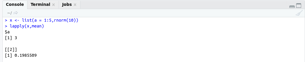
  ############## lapply example #####################

  x <- list(a = 1:5,rnorm(10))
  lapply(x,mean)
OutPut:
Anonymous function
Anonymous functions are those functions that have no name.
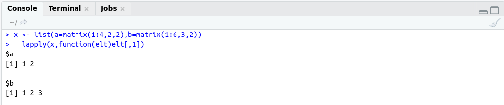
  ############## lapply example #####################
  # Extract first column of matrix


  x <- list(a=matrix(1:4,2,2),b=matrix(1:6,3,2))
  lapply(x,function(elt)elt[,1])
OutPut:
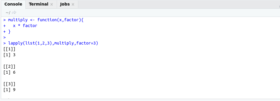
Use function with lapply
  ############## lapply example #####################
  # multiply each element of list with factor


  multiply <- function(x,factor){
    x * factor
  }

lapply(list(1,2,3),multiply,factor=3)
OutPut:
sapply(): Same as lapply but try to simplify the result.
Example:
  ############## sapply example #####################
  # multiply each element of list with factor

  multiply <- function(x,factor){
    x * factor
  }
sapply(list(1,2,3),multiply,factor=3)
OutPut:

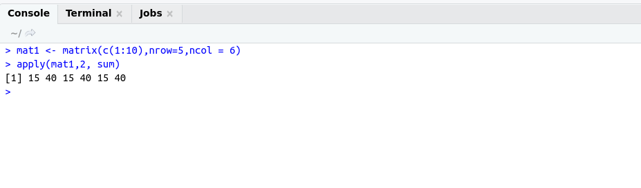
apply() : Apply a function over the margin of an array.
Example:
  ############## apply function #####################

  mat1 <- matrix(c(1:10),nrow=5,ncol = 6)
  apply(mat1,2, sum)
OutPut:
tapply(): Apply a function over subsets of a vector.
Example:
  ############## tapply function #####################

  tapply(mtcars$mpg, list(mtcars$cyl, mtcars$am), mean)
OutPut:
mapply():Multivariate version of lapply.
Example: