Category: Text Mining

In this post, we are discussing more about word cloud and stopwords. As in my previous post, some of the user “Paula Darling, Farzad Qassemi, Georgi Petkov” have commented to me on Linkedin that I have missed to use stopwords. I am thankful to them that they have pointed out my mistakes and suggest me correct them. So, In this post at first, I correct my mistake that I have made in my previous post then after that I introduce some more visuals that we have used during generating word clouds.

So, we are starting from removing stopwords then after that, we will cover these topics:

• Use color function
• Use multiple colors for creating word cloud
• Use prebuilt color palettes

Some More functions that are generally used for text mining

Function	Description
dist()	Compute differences between each row of TDM.
hclust()	Perform cluster analysis on dissimilarities of the distance matrix.
dendrogram()	Visualize the word frequency distances.
plot()	Similar to dendrogram.

Use prebuilt color palettes

viridisLite package

viridisLite color schemes are perceptually-uniform, both in regular form and also when converted to black-and-white, and can be perceived by readers with all forms of color blindness.

The color scales

The package contains four color scales: “Viridis”, the primary choice, and three alternatives with similar properties, “magma”, “plasma”, and “inferno.”

These color palettes are very important during using color scheme and each with a convenience function. Simply specify n to select the number of colors needed.

 

I am not going deep inside viridisLite package because at this moment it is not our priority to learn about viridisLite package but also we have to learn how to use this package to make our visuals more effective during text-mining. 

 

Before going deep inside Word cloud, we first introduce ourselves from some important technical words, that we will use during this word cloud session in text mining .

Basically, the foundation of Bag Word testing is either TDM (Term Document Matrix) or DTM (Document Term matrix).

TDM (Term Document Matrix): The TDM is often the matrix used for language analysis. This is because you likely have more terms than authors or documents and life is generally easier when you have more rows than columns. So, In case of TDM word is represented as row and Document as Column.

 

Each Corpus word is represented as row and Document as Column.

 

How to create TDM from corpus?

TDM Function	Description
TermDocumentMatrix()	Create Term Document Matrix

DTM (Document Text Matrix): Transpose of TDM  hence Document is a row, and each corpus is column.

 

How to create DTM from corpus?

DTM Function	Description
DocumentTermMatrix()	Create Document Term Matrix

Note: Among TDM and DTM which we going to use in our application that depends on scenario that either we want to take terms as a row as rows and document as column then, in that case, we have to pick TDM (Term Document Matrix) and vice-versa we have to focus on DTM (Document Term Matrix).

What is Word Cloud?

Word cloud is Text mining technique that allows us to highlights the most frequent keywords in paragraphs of text.

How to Create a Word Cloud?

There is a simple way for creating word cloud using packages like

tm: for creating corpus and cleaning data.

worldcloud: for constructing word cloud.

Steps for creating Word Cloud :

1. 1. Choose Text file
   2. Install packages and importing packages
   3. Reading file
   4. Converting a text file into corpus
   5. Clean Data and for that execute some commands
   6. Create a Term Document matrix
   7. Create your first cloud

Now without wasting our time we will follow the steps that we have discussed previously and achieve our target to construct word cloud. So, follow the steps

Choose Text file

At first, we choose a text file I have already taken a file that contains speeches of Indian Prime Minister Narendra Modi I will attach this file for you so, that you can be able to practice with it.

Install Packages and importing packages

Install these packages for constructing cloud word for installing these packages you can use install.package() command like this way

#install packages 
Install.packages(‘tm’)
Install.packages(‘wordcloud’)
Install.packages(‘RcolorBrewer’)
#load libary
library(‘tm’)
library(‘wordcloud’) 
library(‘RcolorBrewer’)

Reading file

After installing and loading the library at first, we have need our text data on which we have to process. So, for loading text file and reading data, we will use these commands

# text file location
textFileLocation <- "F:\\Blog\\TextMining\\Word_word_text_mining\\text_speeches\\pm-modi-interacts-with-the-indian-community-in-kobe-japan.txt";
# load text file
textName <- file(textFileLocation,open="r")
# read text file
text_data <- readLines(textName)

Converting a text file into corpus

We can’t directly get word cloud directly from a text file but for constructing word cloud we have to at first convert our text data into the corpus. We can only on corpus for constructing word cloud. So, for constructing word cloud we follow these steps as we had also discussed in our previous post also.

Note: In this case, we are creating Vector Corpus for creating a word cloud.

# create corpus from text_data
textAsCorpus <- VCorpus(VectorSource(text_data)) 

Clean Data and for that execute some commands

Data cleaning is a more important part of any type of Data processing in this case also it is a very important part. For creating cleaning our corpus, we will execute these following commands

# corpus cleaning
clean_text <- tm_map(textAsCorpus,stripWhitespace)
clean_text <- tm_map(textAsCorpus,tolower)
clean_text <- tm_map(textAsCorpus,removeNumbers)
clean_text <- tm_map(textAsCorpus,removePunctuation)

Create a Term Document matrix

This is not a required step because we are considering corpus during creating a word cloud, but in this, I am showing you to calculate Term Document Matrix also.

#creating term Document matrix
tdm1 <- TermDocumentMatrix(clean_text)
# print term document message
print(as.matrix(tdm1))

OutPut:

Create your first Word cloud

It is our final step for creating a word cloud. Now we have to use simple word cloud function of WordCloud package and add corpus inside function.

# create word cloud
wordcloud(clean_text, max.words = 500, colors = "blue")

OutPut:

Complete code

#install packages 
Install.packages(‘tm’)
Install.packages(‘wordcloud’)
Install.packages(‘RcolorBrewer’)
#load libary
library(‘tm’)
library(‘wordcloud’) 
library(‘RcolorBrewer’)

# text file location
textFileLocation <- "F:\\Blog\\TextMining\\Word_word_text_mining\\text_speeches\\pm-modi-interacts-with-the-indian-community-in-kobe-japan.txt";
# load text file
textName <- file(textFileLocation,open="r")
# read text file
text_data <- readLines(textName)

# create corpus from text_data
textAsCorpus <- VCorpus(VectorSource(text_data)) 
# corpus cleaning
clean_text <- tm_map(textAsCorpus,stripWhitespace)
clean_text <- tm_map(textAsCorpus,tolower)
clean_text <- tm_map(textAsCorpus,removeNumbers)
clean_text <- tm_map(textAsCorpus,removePunctuation)

#creating term Document matrix
tdm1 <- TermDocumentMatrix(clean_text)
# print term document message
print(as.matrix(tdm1)) # this not required so we can also comment

# create word cloud
wordcloud(clean_text, max.words = 500, colors = "blue")

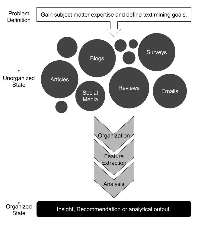
In previous post we had discussed about basic of text mining in R then after that we had little bit talked about Corpus and its types i.e.

1. PCorpus
2. VCorpus

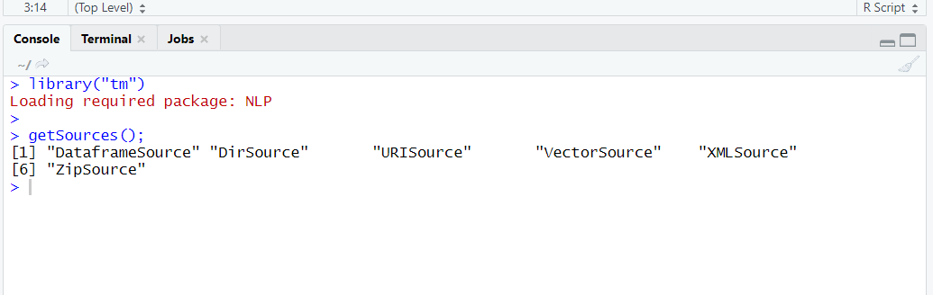
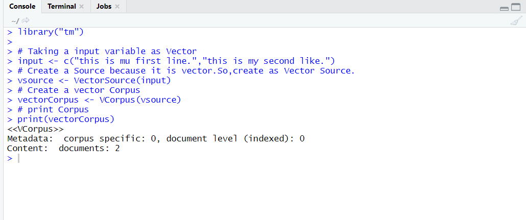
Then in case of VCorpus we understood it’s Sources like VectorSource, DirSource and DataFreameSource we had already explained VectorSource with an Example in this post we are continuing with VCorpus with it’s two remaining sources i.e. DirSource and DataframeSource with example.

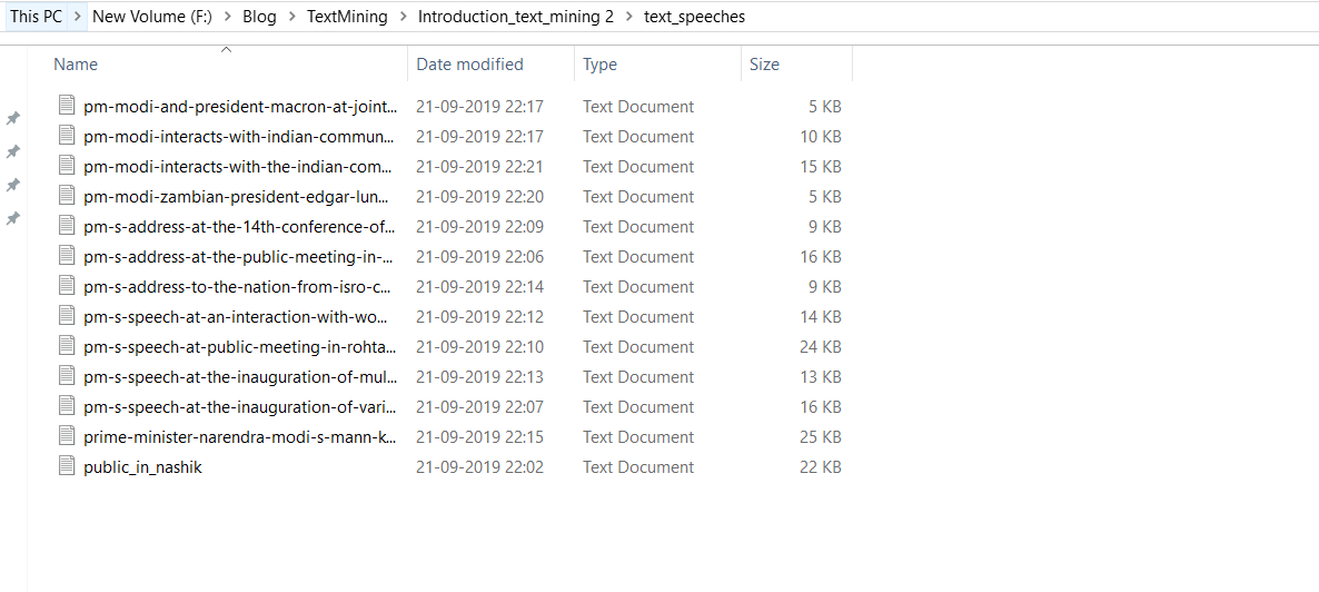
DirSource : It is basically designed for directories on a file system.

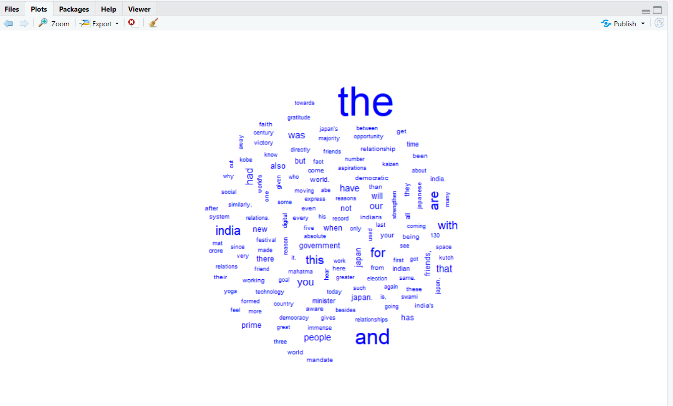
So for further explaining about DirSource we will take a folder which contained some text file I have already created a folder which contains different speeches of Indian Prime Minister Modi I will also share link of this folder so that you can be able to easily download file and practice on it.
Example:

#import tm library
library('tm')
#take file
text <- file.path("text_speeches")
dirSourceCorpus <- VCorpus(DirSource(text))
print(dirSourceCorpus)

DataframeSource : Used for handling data frame csv like structure in this case we are creating our own dataframe example.

Example :

 
#import tm library
library('tm')
# Create a Dataframe example 
example_txt  <- data.frame(
  doc_id=c(1,2,3),
  text= c("example_text","Text analysis provides insights","qdap and tm are used in text mining"),
  author=c("Author1","Author2","Author3"),
  date=c("1514953399","1514953399","1514780598")
)
# Convert DataframeSource frome a example_txt
df_source <- DataframeSource(example_txt)
#Convert df_source to Voletile corpus
df_corpus <- VCorpus(df_source)
#print Voletile Corpus
print(df_corpus)

OutPut :

Some Important functions of TM

TM Function	Description
tolower()	Make all content in lower case
removePunctuation()	Remove Punctuations like period exclamatory
removeNumbers()	Remove Numbers i.e basically use for finding pure text
stripWhiteSpace()	Removing tabs and extra spaces
removeWords()	Removing specific word i.e. defined by Data scientist during process

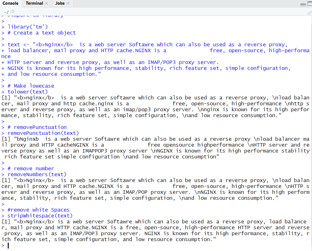
Now it’s time go for example and understand concept in practical way

#import tm library
library('tm')
# Create a text object 
text <- "Nginx  is a web server Softawre which can also be used as a reverse proxy, 
load balancer, mail proxy and HTTP cache.NGINX is a              free, open-source, high-performance 
HTTP server and reverse proxy, as well as an IMAP/POP3 proxy server. 
NGINX is known for its high performance, stability, rich feature set, simple configuration, 
and low resource consumption."
# Make lowecase 
tolower(text)
# removePunctuation
removePunctuation(text)
# remove number
removeNumbers(text)
#remove white Spaces
stripWhitespace(text)

Output :

Like tm package qdap is also very important package for text mining it also contains some important functions that play a vital role during mining

Some of qdap packages are listed here

QDAP Function	Description
bracketX()	Remove all contents within bracket
replace_number()	Replace numbers with their equivalent words like ( 3 becomes three)
replace_abbreviation()	Replace abbreviations with their full text equivalents (e.g. “Er” becomes “Engineer”)
replace_contraction()	Convert contractions back to their base words (e.g. “couldn’t” becomes “could not”)
replace_symbol()	Replace common symbols with their word equivalents (e.g. “$” becomes “dollar”)

Note : Before go for performing qdap example make sure your should contain Java installed.

#import tm library
library('qdap')
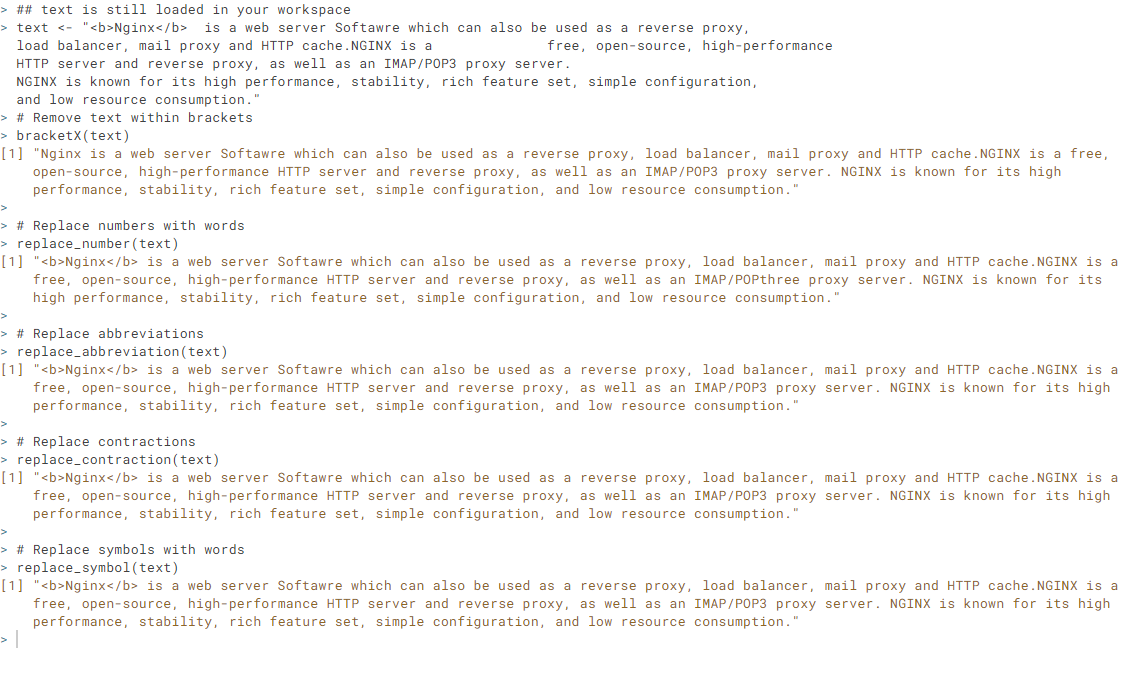
# Create a text object 
text <- "Nginx  is a web server Softawre which can also be used as a reverse proxy, load balancer, mail proxy and HTTP cache.NGINX is a              free, open-source, high-performance HTTP server and reverse proxy, as well as an IMAP/POP3 proxy server. 
NGINX is known for its high performance, stability, rich feature set, simple configuration, and low resource consumption."

# Remove text within brackets
bracketX(text)

# Replace numbers with words
replace_number(text)

# Replace abbreviations
replace_abbreviation(text)

# Replace contractions
replace_contraction(text)

# Replace symbols with words
replace_symbol(text)

Output

Stop Words

Some words come frequently in text and provide little information such type of words are called stop words.In NLP and text mining stop words becomes barrier for our mining or NLP operation.So,during text mining or NLP we remove stop words from our text.

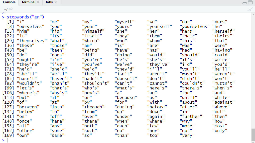
Words like “the”, “a”, “and” are stop words tm packages contains 174 stop words of english. Although you can stop words according to text that we will discuss during practice session.

# import library
library('tm')
# call stopwords function 
stopwords("en")

OutPut:

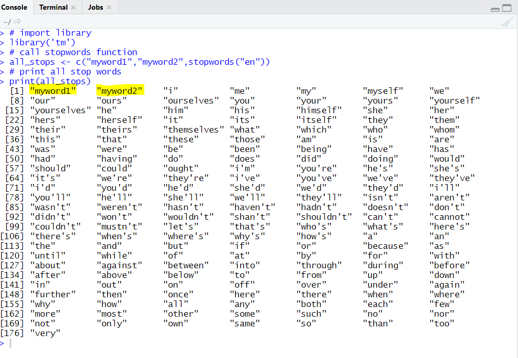
We can also add new stop words in the list stop.

Add new stop words

For adding new stop words inside list we use c() function like for adding two words like “myword1” and “myword2”

Then we will write

# import library
library('tm')
# call stopwords function 
all_stops <- c("myword1","myword2",stopwords("en"))
# print all stop words
print(all_stops)

OutPut : highlighted words are new stop words

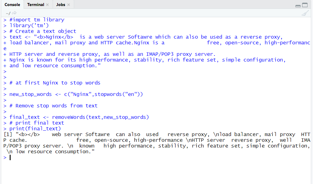
Now it’s time to come when we going to implement stop words concept on real time application.for that purpose we are taking same text  example on which we are considering till yet and from that text file we are removing “Nginx” so “Nginx” is our stop words.

#import tm library
library('tm')
# Create a text object 
text <- "Nginx  is a web server Softawre which can also be used as a reverse proxy, 
load balancer, mail proxy and HTTP cache.Nginx is a              free, open-source, high-performance 
HTTP server and reverse proxy, as well as an IMAP/POP3 proxy server. 
Nginx is known for its high performance, stability, rich feature set, simple configuration, 
and low resource consumption."
# at first Nginx to stop words
new_stop_words <- c("Nginx",stopwords("en")) 
# Remove stop words from text
final_text <- removeWords(text,new_stop_words)
# print final text
print(final_text)

Output:

Word Stemming and Stem Completion

Stemming is a pre-processing step in Text-mining application as well as a very common requirement of Natural Language Processing (NLP) functions.

• Stemming is usually done by removing any attached suffixes and prefixes (affixes) from index terms before the actual assignment of term of index.
• Word Stemming reduces words to unify across documents. for example, the stem of “introducing”, “introduction” and “introduces” is “introduce”.
• During the creation of Stemming it may happen sometimes that we construct such word i.e not real then, in that case, we construct a real word and this process is called stem completion.

Important functions that are used for stemming

TM Stemming function	Description
stemDocument()	Provides root of word.
stemCompletion()	Reconstruct root word.

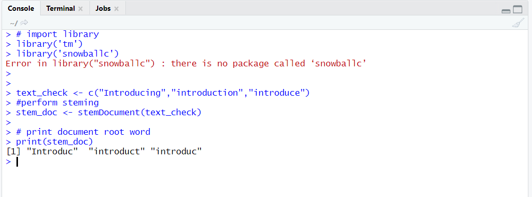
# import library
library('tm')
library('snowballc')
text_check <- c("Introducing","introduction","introduce")
#perform stemming
stem_doc <- stemDocument(text_check)

# print document root word
print(stem_doc)

Output:

Reconstruct word in stemming

# import library
library('tm')
library('snowballc')
text_check <- c("Introducing","introduction","introduce")
#perform stemming
stem_doc <- stemDocument(text_check)
# print document root word
print(stem_doc)
# create introduction dictionary
comp_doc <- "Introduce"
# reconstruct root word
stem_doc_reconstruct <- stemCompletion(stem_doc,comp_doc)
#print reconstruct word
print(stem_doc_reconstruct)

OutPut: